
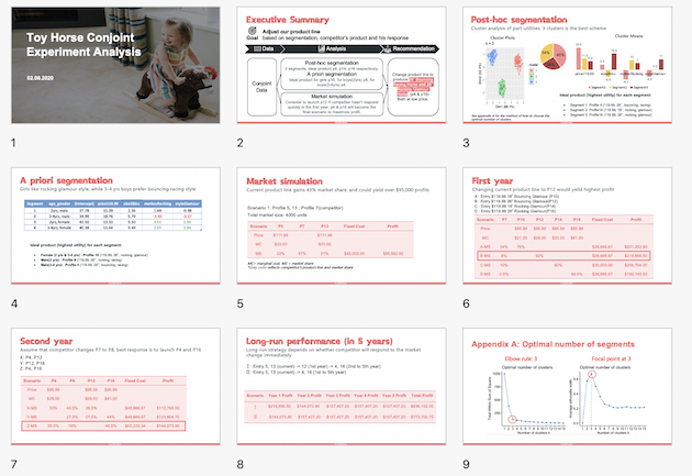
Toy Horse Product Line Revitalization

Summary
- Goal: Provide product portfolio revitalization recommendations to a toy horse company
- Data: Conjoint data of 12 product profiles responded by 200 individuals
- Methodology:
- Use Regression to estimate the conjoint model at the individual level ;
- Conduct Benefit Segmentation via Cluster Analysis of Conjoint Part-Utilities;
- Conduct a priori segmentation using the variables gender and age;
- Simulate market shares for different product-line scenarios.
Scenario
In this project, I worked for a relatively small toy company called EarlyRiders. The company had a recent management change and realized that their product set was underperforming. They currently offer two products and one in particular was not doing well. The management team decided to revitalize their product portfolio based on the opinions of potential end-users. For this purpose, a conjoint analysis was run by the company, and my goal was to analyze the conjoint data and provide product line adjustment recommendations to the management team.
Data
The raw data I have is the conjoint data of 200 individuals consisting of 12 product profiles out of 16. These individuals are made up of parents of 2-4 year old kids who planned to purchase a toy horse.
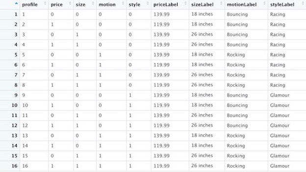
The conjoint study examined four attributes: price, height, motion, and style. The levels for retail price are $119.99 and $139.99, for height are 18" and 26", for motion are rocking or bouncing, and for style are glamorous or racing.
A screenshot of the conjoint data and the profile data shown as below.
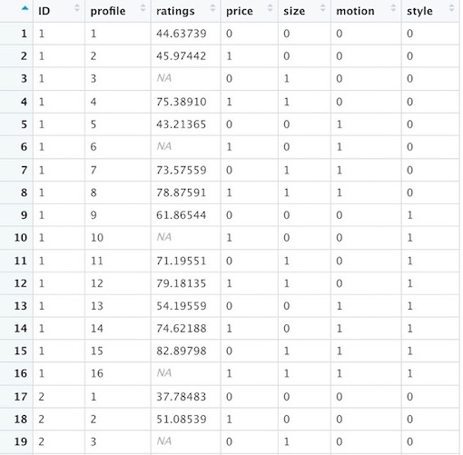
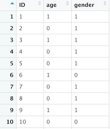
In addition to the conjoint data, the gender and age of the child was recorded (Gender=1 if Female, 0 if Male; Age=0 if 2 years old, 1 if 3-4).
Analysis
Step1. Post-hoc Segmentation via Cluster Analysis of Conjoint Part-Utilities
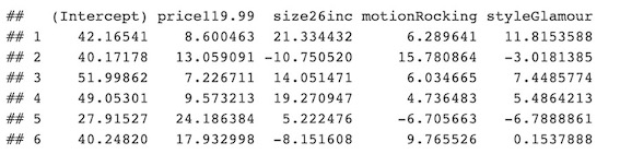
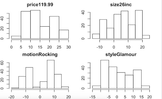
First, I ran regression in R to estimate the conjoint part-utilities at the individual level. The distribution of the part-utilities for each of the four attributes are shown in the graph below.
##### Produce part-utilities #####

coeflist=list()
for(i in 1:200) {
    reg = lm(ratings~factor(price)+factor(size)+factor(motion)+factor(style),
             data=conjointData[conjointData$ID==i,])
    coeflist[[i]] = reg$coefficients
}
partworths = as.data.frame(do.call(rbind, coeflist))
colnames(partworths)[2:5] = c('price119.99', 'size26inc','motionRocking', 'styleGlamour')
head(partworths)

par(mfrow=c(2,2))
par(mar=c(2,2,2,2))
for(i in 2:length(partworths)){
    hist(partworths[,i], main=names(partworths)[i])
}
With the individual-level part-utilities data, I was the able to conduct a Cluster Analysis. In order to find out the optimal number of clusters, I applied the Elbow Rule, which is used within sum of squared errors, and the Silhouette Rule, which measures the overall performance. Both the graphs below show that 3 clusters seem to be a good choice.
##### Choosing the optimal number of clusters #####

library(gridExtra)

clustTest = function(toClust,print=TRUE,scale=TRUE,maxClusts=15,seed=12345,nstart=20,iter.max=100){
    if(scale){ toClust = scale(toClust);}
    set.seed(seed);   # set random number seed before doing cluster analysis
    wss <- (nrow(toClust)-1)*sum(apply(toClust,2,var))
    for (i in 2:maxClusts) wss[i] <- sum(kmeans(toClust,centers=i,nstart=nstart,iter.max=iter.max)$withinss)
    ##gpw essentially does the following plot using wss above.
    #plot(1:maxClusts, wss, type="b", xlab="Number of Clusters",ylab="Within groups sum of squares")
    gpw = fviz_nbclust(toClust,kmeans,method="wss",iter.max=iter.max,nstart=nstart,k.max=maxClusts) #alternative way to get wss elbow chart.
    pm1 = pamk(toClust,scaling=TRUE)
    ## pm1$nc indicates the optimal number of clusters based on
    ## lowest average silhoutte score (a measure of quality of clustering)
    #alternative way that presents it visually as well.
    gps = fviz_nbclust(toClust,kmeans,method="silhouette",iter.max=iter.max,nstart=nstart,k.max=maxClusts)
    if(print){
        grid.arrange(gpw,gps, nrow = 1)
    }
    list(wss=wss,pm1=pm1$nc,gpw=gpw,gps=gps)
}

checks = clustTest(partworths,print=TRUE,scale=TRUE,maxClusts=15,seed=12345,nstart=20,iter.max=100)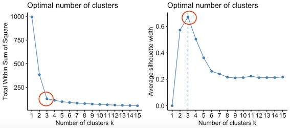
I then further looked at the cluster plots against Principle Components. The graph below clearly showed that 3 clusters would be the best scenario.
##### Choosing the optimal number of clusters #####

##Runs a set of clusters as kmeans
runClusts = function(toClust,nClusts,print=TRUE,maxClusts=15,seed=12345,nstart=20,iter.max=100){
    if(length(nClusts)>4){
        warning("Using only first 4 elements of nClusts.")
    }
    kms=list(); ps=list();
    for(i in 1:4){
        kms[[i]] = kmeans(toClust,nClusts[i],iter.max = iter.max, nstart=nstart)
        ps[[i]] = fviz_cluster(kms[[i]], geom = "point", data = toClust) + ggtitle(paste("k =",nClusts[i]))
    }
    library(gridExtra)
    if(print){
        tmp = marrangeGrob(ps, nrow = 2,ncol=2)
        print(tmp)
    }
    list(kms=kms,ps=ps)
}

clusts = runClusts(partworths,c(2,3,4,11),print=TRUE,maxClusts=15,seed=12345,nstart=20,iter.max=100)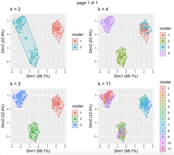
Looking at the 3-cluster scenario in more depth, I found that customers of these three cluster take up 40%, 34% and 26% of the total sample respectively.
##### Benefit Segmentation via Cluster Analysis #####

##Plots a kmeans cluster as three plot report
plotClust = function(km,toClust,discPlot=FALSE){
    nc = length(km$size)
    if(discPlot){par(mfrow=c(2,2))}
    else {par(mfrow=c(3,1))}
    percsize = paste(1:nc," = ",format(km$size/sum(km$size)*100,digits=2),"%",sep="")
    pie(km$size,labels=percsize,col=1:nc)

    clusplot(toClust, km$cluster, color=TRUE, shade=TRUE,
             labels=2, lines=0,col.clus=1:nc); #plot clusters against principal components

    if(discPlot){
        plotcluster(toClust, km$cluster,col=km$cluster); #plot against discriminant functions ()
    }
    rng = range(km$centers)
    dist = rng[2]-rng[1]
    locs = km$centers+.05*dist*ifelse(km$centers>0,1,-1)
    bm = barplot(km$centers,beside=TRUE,col=1:nc,main="Cluster Means",ylim=rng+dist*c(-.1,.1))
    text(bm,locs,formatC(km$centers,format="f",digits=1))
}

par(mar=c(2,2,2,2))
plotClust(clusts[[1]][[2]],partworths)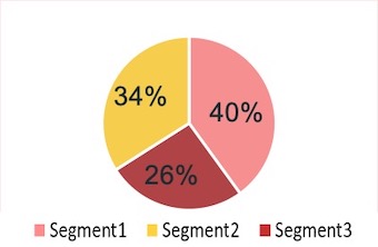
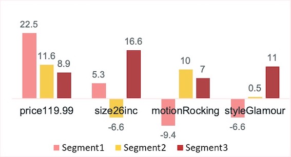
At the same time, these 3 segments show quite different preference for each attribute, which we can see from the attribute utility means for each segment on the graph below. For price, all 3 segments gain higher utility in the lower price of 119.99 dollars, but at different levels. For size, segment 1 and 3 show preference for larger size of 26 inches, while segment 2 gain more utility in smaller size of 18 inches. Similar for the motion and style attributes.
Based on the cluster means, we can find out the ideal product for each of these 3 segments are profile 4,14,16 respectively. The characteristics of each post-hoc segment and detailed profile information are shown in the table below.
| Segment NO. | Characteristics | Ideal Product |
|---|---|---|
| 1 | Price sensitive, bouncing & racing style lover | Profile 4 ($119.99, 26’’, bouncing, racing) |
| 2 | Smaller size & rocking lover | Profile 14 ($119.99, 18’’, rocking, glamour) |
| 3 | Bigger size & glamourous style lover | Profile 16 ($119.99, 26’’, rocking, glamour) |
Step2. A priori Segmentation using Gender and Age
Next, I conducted a priori segmentation using the variables age and gender, which generated four different segments. Based on the segment-level regression results, we can confirm the preference difference of different age and gender groups.
##### A priori Segmentation with age_gender#####

coeflist=list()
for(i in 1:4) {
    reg = lm(ratings~factor(price)+factor(size)+factor(motion)+factor(style),
             data=merge_conjointData[merge_conjointData$age_gender==i,])
    coeflist[[i]] = reg$coefficients
}
age_gender_partworths = as.data.frame(do.call(rbind, coeflist))
colnames(age_gender_partworths)[2:5] = c('price119.99', 'size26inc','motionRocking', 'styleGlamour')
age_gender_partworths$age_gender = c('2yrs,male','3-4yrs,male','2yrs,female','3-4yrs,female')
age_gender_partworths
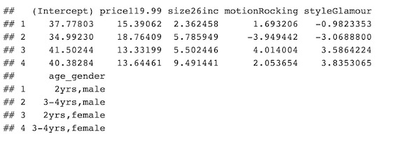
From the table above, we can see that girls show clear preference for rocking horse and glamorous style, while 3-4 year-old boys have higher utility in bouncing horse and racing style. We can also see that 2 year-old boys or girls have higher utility for rocking horse than the 3-4 year-olds.
As for price and size, all 4 segments show high utility for lower price and bigger size, but at different levels. Girl on average have a higher utility for bigger size than boys. Both 3-4 year-old boys and girls prefer bigger size than their 2 year-old counterparts, which is quite intuitive given their age difference.
According to these findings, we can tell the ideal product of these 4 segments are profile 4,8,16.
| Segment | Ideal Product |
|---|---|
| Male(3-4 yrs) | Profile 4 ($119.99, 26’’, bouncing, racing) |
| Male(2 yrs) | Profile 8 ($119.99, 26’’, rocking, racing) |
| Female(2 yrs & 3-4 yrs) | Profile 16 ($119.99, 26’’, rocking, glamour) |
Step3. Market Shares Simulation
After analyzing the customer segmentation, I ran several market simulations to determine the ideal product portfolio for the company in order to maximize the profit.
1. Current Scenario
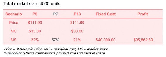
Based on the conjoint data for different profiles, we can calculate the market share under different market scenarios and also the profit using given cost information. Currently the company launched 18 inches Rocking Glamour and the same size Rocking Racing horse at $119.99, which are Profile 5 and 13; while our competitor sells 26’’ Racing Rocking Horse at $139.99, which is Profile 7. Calculation results are shown in the chart below: now our two products account for 43% of total market share, yielding a profit of $95,000+ per year.
2. First Year
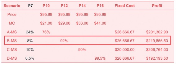
I then tried some other profiles for simulation. While it is a waste of time running all combinations of 16 profiles, I first selected Profiles 10, 12, 14 and 16, which have a lower price of $119.99, to replace our current ones. The reason is that from previous research we found consumers are price sensitive, and these four profiles are most likely to expand our market share. Assume the competitor keeps launching profile 7, changing product line to 26’’ Bouncing Glamour toy horse could gain highest market share and profit, which is nearly $220,000 per year; while our competitor’s market share would decrease to only 8% in this year.
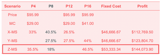
3. Second Year
Given the competitor’s information, we know that our competitor would not change the product offering, but might respond by lowering price after the first year’s loss in market share.
Therefore, I assumed the competitor changed from launching profile 7 to profile 8 in the second year. In this case, it’s reasonable to launch as many popular products as possible to shrink the competitor’s market share. Based on the result of our previous research of segmentation, profile 4 and 16 are the most popular toy horses and preferred by most children. Combining profile 4 and 16 with profile 12 that we launched in the first year, I rearranged these three profiles into three combinations X, Y and Z. Among these three combinations, Z has highest market share and largest profit. Therefore, launching profile 4 and 16 is the best scenario for the second year.
4. Long Run Consideration
Company’s long-run strategy would depend on whether competitor would respond to the market change immediately. If he didn’t respond until the second year as we expected, then the optimal revitalization plan for the company would be to change from Profiles 5, 13 to Profile 12 in the first year, and to Profiles 4, 16 after (26” Bouncing Racing Horse and 26” Rocking Glamour Horse.).
#####  Market Share Simulation #####

simFCDecisions = function(scen,data){
    inmkt = data[,scen] #construct the subsetted matrix of options
    retlist=list()
    for(i in 1:nrow(inmkt)){
        maxvalue=max(inmkt[i,])
        testmax=as.numeric(inmkt[i,]==maxvalue)
        summax=sum(testmax)
        ret=testmax/summax
        retlist[[i]]=ret
    }
    ret = as.data.frame(do.call(rbind, retlist))
    names(ret) <- names(inmkt)
    ret
}
calcUnitShares = function(decisions){
    colSums(decisions)/sum(decisions) #assumes that total decisions is market size
}
simFCShares=function(scen,data){
    decs = simFCDecisions(scen,data) #determine decisions
    calcUnitShares(decs) #calculate shares and return
}
simFCScenarios = function(scenarios,data,...){
    res = matrix(nrow=length(scenarios),ncol=length(data)) #sets everything to NA by default
    for(i in 1:length(scenarios)){ ##loop over scenarios
        res[i, scenarios[[i]] ] = simFCShares(scenarios[[i]],data,...)##  calculate market shares and save to right columns in res for the scenario
    }
    res = as.data.frame(res); names(res) = names(data)
    res ##return result table
}

### Profitablity anlysis
# assign cost
profilesData$vc <- c(rep(c(21,21,29,29,33,33,41,41),2))  # variable cost of each profile
profilesData$wsprice <- c(rep(c(111.99,95.99),8)) # wholesale price of each profile
profilesData$margin <- profilesData$wsprice - profilesData$vc # contribution margin of each profile

simMargin = function(scen,data){ # calculate margin for each scenario
    shares=simFCShares(scen,data)
    margin=c()
    for (i in 1:length(scen)){
        margin <- c(margin,shares[i]*profilesData$margin[profilesData$profile == scen[i]]*4000)
    }
    margin
}
simMarginScenarios = function(scenarios,data,...){
    res = matrix(nrow=length(scenarios),ncol=length(data)) #sets everything to NA by default
    for(i in 1:length(scenarios)){ ##loop over scenarios
        res[i, scenarios[[i]] ] = simMargin(scenarios[[i]],data,...)##  calculate margin and save to right columns in res for the scenario
    }
    res = as.data.frame(res); names(res) = names(data)
    res ##return result table
}

### Set up scenarios
scens = list()
scens[[1]]=c(5,7,13) #  status quo: own product p5 & p13, competitor p7
# first year scenarios
scens[[2]]=c(7,10) # competitor p7(not change) + own p10
scens[[3]]=c(7,12) # competitor p7(not change) + own p12 - profit max
scens[[4]]=c(7,14) # competitor p7(not change) + own p14
scens[[5]]=c(7,16) # competitor p7(not change) + own p16
# second year scenarios
scens[[6]]=c(4,8,12) # competitor change to p8 + own p12 plus p4
scens[[7]]=c(8,12,16) # competitor change to p8 + own p12 plus p16
scens[[8]]=c(4,8,16) # competitor change to p8 + own change to p4 & p16 - profit max


### Market share and contribution margin for all scenarios
simFCScenarios(scens,ratingData_wide[,2:17])  # market share
simMarginScenarios(scens,ratingData_wide[,2:17]) # contribution margin
Final Report
Key Words: R, Conjoint Analysis, Cluster Analysis, Benefit Segmentation, Market Simulation